Distributed Decision Trees with Heterogeneous Parallelism
Alex Xiao (axiao@andrew.cmu.edu)
Rui Peng (ruip@andrew.cmu.edu)
Final Report
Summary
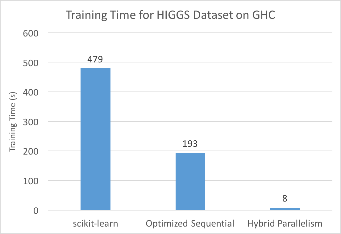
Decision tree learning is one of the most popular supervised classification algorithms used in machine learning. In our project, we attempted to optimize decision tree learning by parallelizing training on a single machine (using multi-core CPU parallelism, GPU parallelism, and a hybrid of the two) and across multiple machines in a cluster. Initial results show performance gains from all forms of parallelism. In particular, our hybrid, single machine implementation on GHC achieves an 8 second training time for a dataset with over 11 million samples, which is 60 times faster than scikit-learn and 24 times faster than our optimized sequential version, with similar accuracy.
Background
Decision Tree Basics
Decision trees are a common model used in machine learning and data mining to approximate regression or classification functions. They model functions of the form:
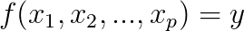
Where x1 through xp are the features of the input and y is the output.
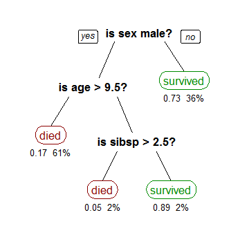
A decision tree models this function with a series of queries of the form “xi > v?”, where v is a value of the feature. For example, below is an example of a decision tree used to predict whether or not a passenger survived the Titanic, based on the features gender, age, and number of siblings/spouses.

For the purposes of this project, we will focus on classification decision trees, where we are trying to predict the class label of an input, such as in the example above.
Building the Decision Tree
Decision tree training algorithms learn by training on examples in the form of (x1,x2,…,xn,y). While building the tree, decision tree training algorithms would need to create nodes that represent a query of the form “xi > v?”. The root node initially contains all of the data, and when the decision tree chooses the query, or the split point, the data is partitioned into left and right children. This process repeats until the tree has sufficient size, and the class label assigned to the leaves of the tree can simply be the majority class label of the data assigned to the leaf.
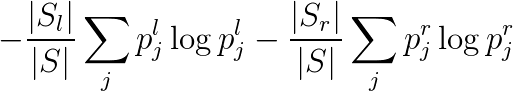
Typically the most computationally expensive portion of this process is evaluating the potential split points for each feature. The evaluation for a split point is usually based on some kind of metric that captures the distribution of the class labels of the data after the split. For example, a common criteria to use is the minimum weighted entropy of the children nodes, which is defined below. Sl is the size of left child’s data partition and plj is the fraction of the left child’s data partition that has class label j. Variables for the right child are defined similarly.
When the feature values are continuous, it is more efficient to compute this weighted sum for each split point by first sorting the values based on each feature and scanning through the sorted list. This way we can maintain the left and right distributions of the class labels and evaluate all split points for a feature in one scan. Below is pseudo-code for how a decision tree training algorithm that achieves this.
// root contains all the data
work_queue.add(root)

while (!work_queue.empty()) {
  node = work_queue.remove_head()

  if (node.is_terminal()) continue

  best_split_point = nil

  for f in features {
    sort(node.data, comparator = f)

    left_distribution = empty()
    right_distribution = node.get_distribution()

    for d in node.data {
      // check this split point based off some criteria, like entropy
      criteria = eval(left_distribution,right_distribution)

      best_split_point = upate_best_split_point(criteria, best_split_point)
      update_distributions(left_distribution, right_distribution, d);
    }
  }

  // partition data based on split point
  left,right = split(node, best_split_point)

  work_queue.add(left)
  work_queue.add(right)
}
A Faster Sequential Algorithm
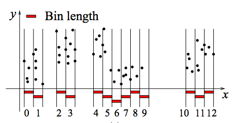
Unfortunately, the standard decision tree construction algorithm is slow even for sequential standards, since repeated sorting of data becomes a bottleneck. One common optimization for this is to first pre-process the dataset by constructing a histogram for each feature to compactly describe the distribution of the data.
With these histograms, sorting is no longer necessary. Below is pseudo-code of how to leverage the histogram binning technique.
root.histograms = construct_histograms()
work_queue.add(root);

while (!work_queue.empty()) {
  node = work_queue.remove_head()

  if (node.is_terminal()) continue

  best_split_point = nil

  for f in features {
    left_distribution = empty()
    right_distribution = node.get_distribution()

    for bin in node.histograms(f) {

      // check this split point based off some criteria, like entropy
      criteria = eval(left_distribution,right_distribution)

      best_split_point = upate_best_split_point(criteria, best_split_point)
      update_distributions(left_distribution, right_distribution, bin);
    }
  }

  left,right = split(node, best_split_point)
  left.compute_histograms(node.histogram, best_split_point)
  right.compute_histograms(node.histogram, best_split_point)

  work_queue.add(left)
  work_queue.add(right)
}
This eliminates data sorting and also scans over histogram bins instead of data points. Since number of bins (set to a constant value like 255), which is much less than the number of datapoints. This should provide a big performance gain when searching for split points. The main computation is now offloaded to building the initial histograms and constructing new histograms from old histograms. Our efforts in this project were to use parallelism to accelerate these two parts. Specifically, we were interested to see how fast we could make this algorithm by using all the different computational resources available here to us at CMU, which include multi-core CPUs, GPUs, and a distributed cluster.
Challenges
To summarize, these are the challenges we face in this project:
-
Building an optimized sequential implementation of decision tree learning to use as a baseline requires some work, since the default decision tree training algorithm is slow and requires repeatedly sorting the dataset, which can be massive.
-
Parallelizing training with a machine on CPU cores is also tricky, since the shape of the decision tree is irregular and determined at runtime, making static partitioning of the workload across tree nodes ineffective.
-
Distributing training across machines in a cluster requires significant communication between machines, since the decision on which feature to split on requires a global view of the dataset.
-
The standard algorithm for decision tree learning does not translate well to GPU or hybrid implementations. To quote the creator of XGBoost, a widely used decision tree boosting framework: “The execution pattern of decision tree training relies heavily on conditional branches and thus has high ratio of divergent execution, which makes the algorithm have less benefit from SPMD architecture”. Our implementation of decision tree learning must not have the same problems.
-
Scheduling GPU and CPU computation on a heterogeneous machine is difficult, since it is crucial to identify scenarios in which one is preferred over the other or if the overhead of using both is worth the trouble.
Approaches and Results
As we seek to optimize the performance of the algorithm using all the techniques we learned in class and leverage different computing hardware, we describe our approaches and results for individual optimizations.
Optimizing a Sequential Implementation
Approach
We first implemented the naive, sorting based implementation for decision tree training. After some initial profiling, we then implemented the histogram-based algorithm mentioned above.
To construct the initial histogram bins efficiently, we implemented an adaptive histogram construction algorithm based on this paper. We also optimized the histogram splitting phase by only reconstructing the smaller child’s histograms when we split a node. The larger child’s histogram can then be quickly constructed from its parent’s and its sibling’s histograms through histogram subtraction.
Result
Below are performance comparisons between our implementations of the sorting-based algorithm and the histogram-based algorithm. We also compare our performance with a popular framework used for decision tree training: scikit-learn. We benchmarked on the Microsoft Learning to Rank dataset, which contains 2 million (query, url) pairs, each with 136 features and a label denoting the relevance of the query to the url. Experiments were performed on GHC. We set the maximum number of leaves in the decision tree to be 255, which is consistent with all experiments listed on this page.
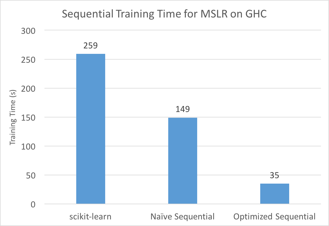
Our final sequential version observes massive improvements over both scikit-learn and the traditional decision tree learning algorithm, for the reasons mentioned in Background. This is the optimized sequential version we will use as a baseline later. Note that although our accuracy has also decreased slightly due to the approximate nature of our histogram binning, the reduction is small (around 0.05%) and is not much of a concern if we used our algorithm in an ensemble method (which people often do with decision trees). Furthermore, since our focus is on performance, we decided to not spend too much time on sophisticated splitting heuristics and pruning techniques that are found in mature frameworks as long as our accuracy is competitive.
Parallelizing with Multiple CPU Cores
Approach
As mentioned previously, parallelizing across tree nodes suffers from the problem of an imbalanced workload. Instead, we decided to parallelize the decision tree training algorithm within a single tree node, specifically for the two expensive areas as mentioned previously:
- Initial building of histograms.
- Splitting parent histograms into child histograms.
We used OpenMP to parallelize these two areas across features. Since building histograms and constructing child histograms requires scanning over the distributions of every histogram bin of every feature, this should lead to a roughly balanced workload.
Result
The graph below shows the training times of the parallel algorithm run on different numbers of threads. Experiments were performed on GHC and the Microsoft Learn to Rank dataset.
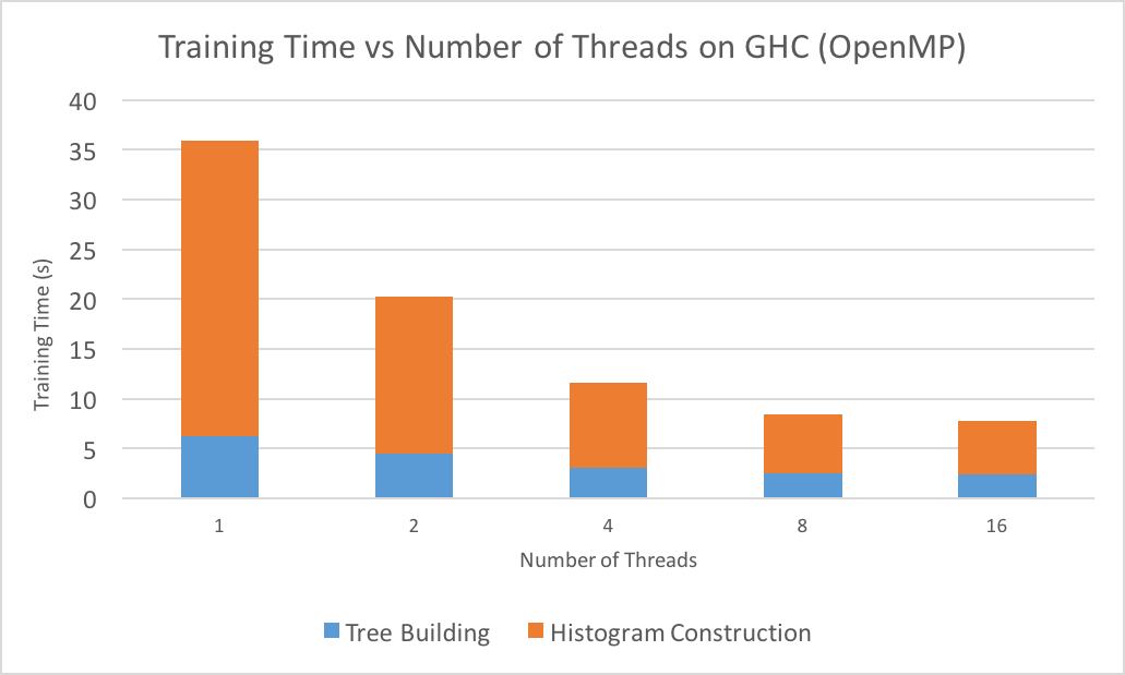
The graph above at first displays near-linear speedup, especially for histogram construction across different features. We suspect that the eventual dissipation of speedup is very likely due to maxing out on memory bandwidth, since parallelizing histogram construction across features needs minimal synchronization but requires accessing a lot of memory. To solve this problem, we decided to utilize more resources available to us here at CMU, such as distributed cluster machines on Latedays and GPUs on GHC machines.
Distributing Training with Multiple Machines
Approach
The communication efficiency of distributed training was a major concern we had initially, but is somewhat alleviated by our histogram representation of the dataset. This allows multiple machines to communicate with histogram statistics instead of their the full dataset statistics, drastically reducing the communication requirements.
Our first distributed algorithm roughly works as follows:
-
Each machine in the cluster is assigned a partition of the dataset. One machine is designated as the master which will be responsible for evaluating split points.
-
Each machine initially constructs local histograms of their partition and assigns their local root node the histograms like before.
-
While there are still nodes to be split, each worker sends their local histograms for each feature for that node to master. Master merges these histograms and evaluates possible split points like before.
-
Master sends the best split point to the workers. Each machine in parallel now splits the node into left and right children. Repeat steps 3 and 4 as needed.
The parallelism that we gain from this algorithm is that each machine can construct and maintain histograms for their partition in parallel. Evaluating possible split points accurately, however, requires a global view of the feature distributions and as a result, master needs all the histograms to make a decision. This could result in high communication overhead, since every node we split in the decision tree would require this information exchange.
Our second distributed algorithm attempted to fix this problem by minimizing communication efficiency through an algorithm recently published in a paper at NIPS. The idea is to maximize local computations on each worker before communicating with master. The algorithm is now roughly as follows (steps 1 and 2 same as before):
-
While there are still nodes to be split, each worker first uses their local histograms to evaluate possible split points.
-
Each worker votes for their top k features, where k is a configurable parameter.
-
Master aggregates the votes and requests the top 2*k most voted features.
-
Workers send their local histograms for the top 2*k features to master. Master merges these histograms and evaluates possible split points like before.
-
Master sends the best split point to the workers. Each machine in parallel now splits the node into left and right children. Repeat steps 3 to 7 as needed.
We implemented the above algorithms with Open MPI for communication between master and worker and OpenMP for parallelism within a machine like before.
Result
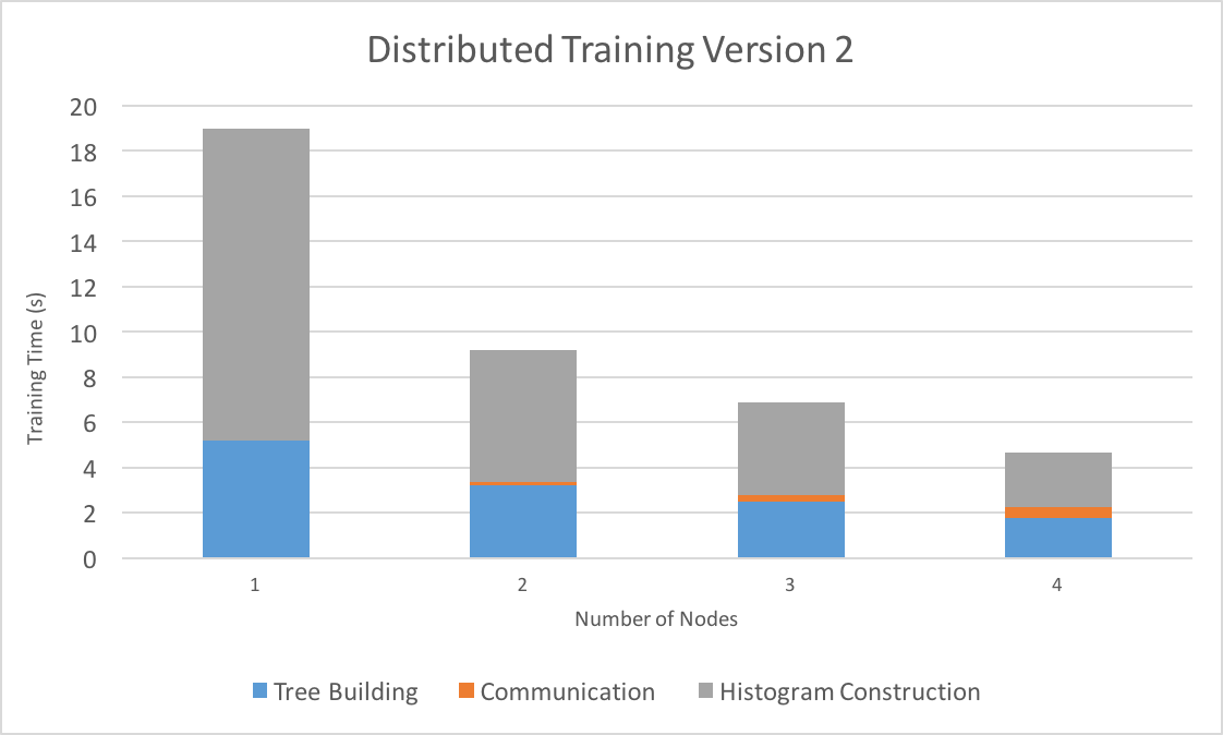
We evaluated the two algorithms on the Latedays cluster with a varying number of nodes, with k = 5 for our distributed voting algorithm. We again used the Microsoft Learn to Rank dataset (2 million samples, 136 features) to evaluate training time.
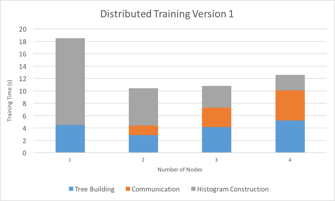
In the first graph, which shows training times for the first distributed algorithm, we can see that distributing training with 2 nodes gives us good speedup. Communication time, however, starts to dominate after 2 nodes such that total training time actually starts to increase. The time to actually construct the tree goes up as well, since with more nodes there are more split points to consider, outweighing the advantages we get from parallelizing histogram construction and splitting.
In the second graph, which shows training times for the second distributed algorithm, we can see that the voting scheme reduces communication and tree building time drastically, leading to good scaling beyond just 2 nodes. When run on 4 nodes, training finishes in 4.66 seconds, which is about a 4x speedup over running on 1 node (all nodes are also running OpenMP code with 24 threads).
Since there is no guarantee that the local information used to pick feature candidates for splitting actually included the globally best feature, the distributed voting scheme is an approximation. To make sure our implementation did not sacrifice accuracy for speed, we also measured the accuracy of our trained decision tree as we scaled the number of nodes. We also compared the accuracy of our distributed algorithm with a sequential scikit-learn implementation.
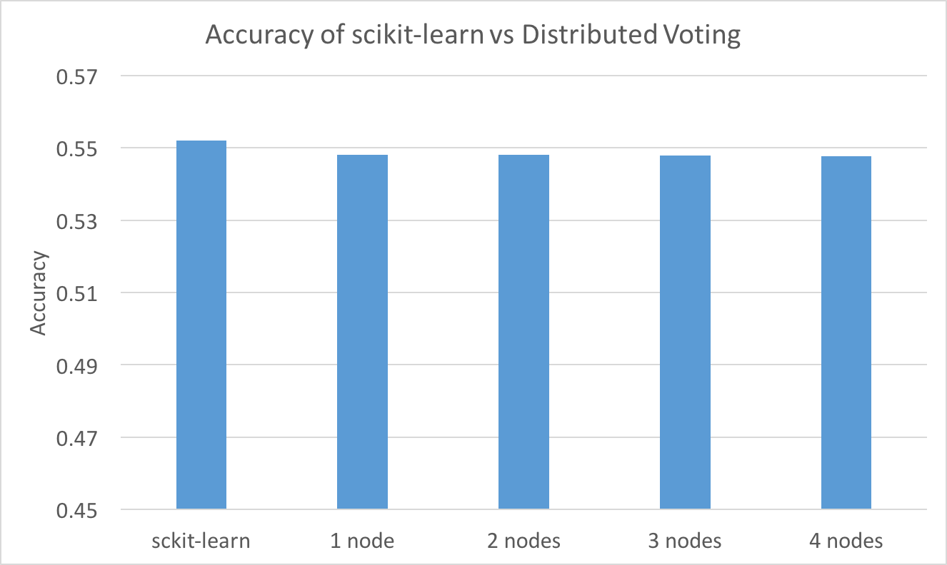
As the number of nodes increases, accuracy hardly changes at all, which suggests that this approximation is robust (the theoretical soundness is also proved in the original paper).
GPU and Hybrid Implementation
Approach
Another advantage of our histogram implementation is that the main bottleneck during
tree construction is computing child histograms, which requires a lot of memory
movement and updates. This kind of computation lends
itself well to a GPU implementation. We use CUDA kernels to perform updates of histogram bin
statistics. Each CUDA thread block is assigned to a feature, in which all CUDA threads
update histogram bin distributions by looping over
data points within the tree node in an interleaved fashion. To further reduce global
memory writes we allocate a local __shared__ buffer to do local updates
and push the agreggate updates to global memory at the end.
As an extension of using only GPU to perform histogram updates and letting CPU stay idle, we further improve performance by adopting a hybrid algorithm – specifically we assign different features to CPU and GPU to perform histogram updates (see pseudo-code below). The workload nature of histogram updating is easily dividable to CPU and GPU since updates to different features will be written to different locations without any data races. The key advantage of scheduling work to CPU and GPU is that we can perform asynchronous CUDA kernel calls and utilize both types of compute hardware to do work in parallel.
gpu_features, cpu_features = assign_features(features)
gpu_result = []
cpu_result = []

// Asynchronously compute on gpu
kernel_gpu_compute_histograms(gpu_features, gpu_result)

cpu_compute_child_histograms(cpu_features, cpu_result)

cudaThreadSynchronize()

merge_results(gpu_result, cpu_result)
Result
Since the speedup graph for CPU suggests that our algorithm may be bandwidth bound, an implementation that uses both the memory bandwidth of GPU and CPU will likely be faster. When run on the Microsoft Learning to Rank dataset on GHC, we found that hybrid reduces tree building time by 10% (note: this does not include initial histogram construction, which we did not accelerate with GPUs).
For each tree node, we chose to assign 8 features to CPU and the rest to GPU as our GPU/CPU hybrid assignment. We then used a dynamic scheduling policy which used the hybrid version for nodes with more samples and CPU-only for nodes with fewer samples (much like choosing between top-down and bottom-up in hybrid BFS in assignment 3). This dynamic scheduling tries to minimize data transfer between GPU and CPU in cases where doing work on GPU is not worth the data transfer overhead.
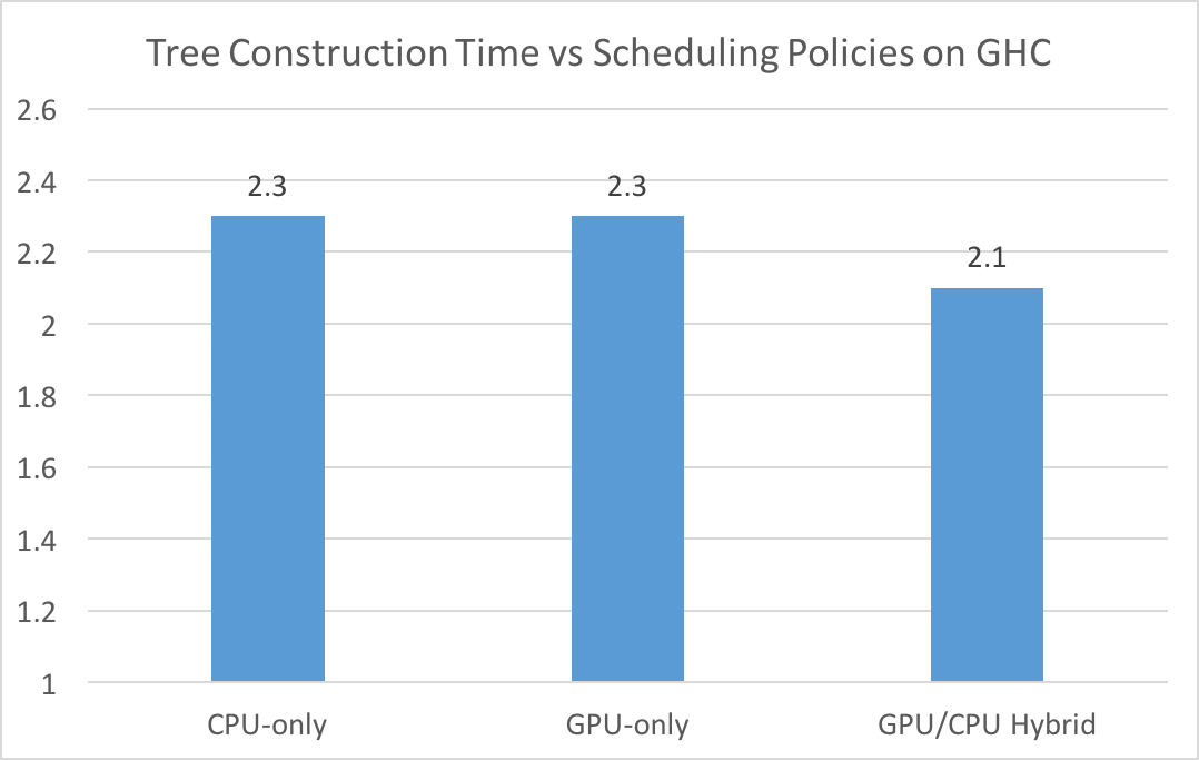
With this scheme, the dynamic hybrid version out-performs the GPU-only and the CPU-only versions by a decent margin by utilizing heterogeneous computing resources. It is interesting that CPU-only and GPU-only have the same runtime. After profiling, we found that the initial CUDA memory setup time (cudaMalloc, initial cudaMemcpy’s) takes up 25% of total tree construction time, which makes the overall runtime of GPU-only the same as CPU-only despite the relatively fast CUDA kernel calls used to compute child histograms. This indicates that to find a good hybrid scheduling strategy, we need to carefully profile the code and place the work optimally on GPU and CPU depending on specific workload conditions. If we had more time for the project, we would perform a more comprehensive profiling and devise an optimal dynamic scheduling policy.
Although we didn’t have time to devise a better dynamic scheduling policy, we did some initial testing of hybrid on a larger dataset. Since we suspected that the overhead of CUDA memory setup time was limiting the advantages of hybrid/GPU, we tried running our hybrid algorithm on the HIGGS dataset, which contains 11,000,000 samples. We ran our hybrid algorithm against sequential versions of the algorithm and compared its speedup when run on the Microsoft Learning to Rank dataset (about 2,000,000 samples).
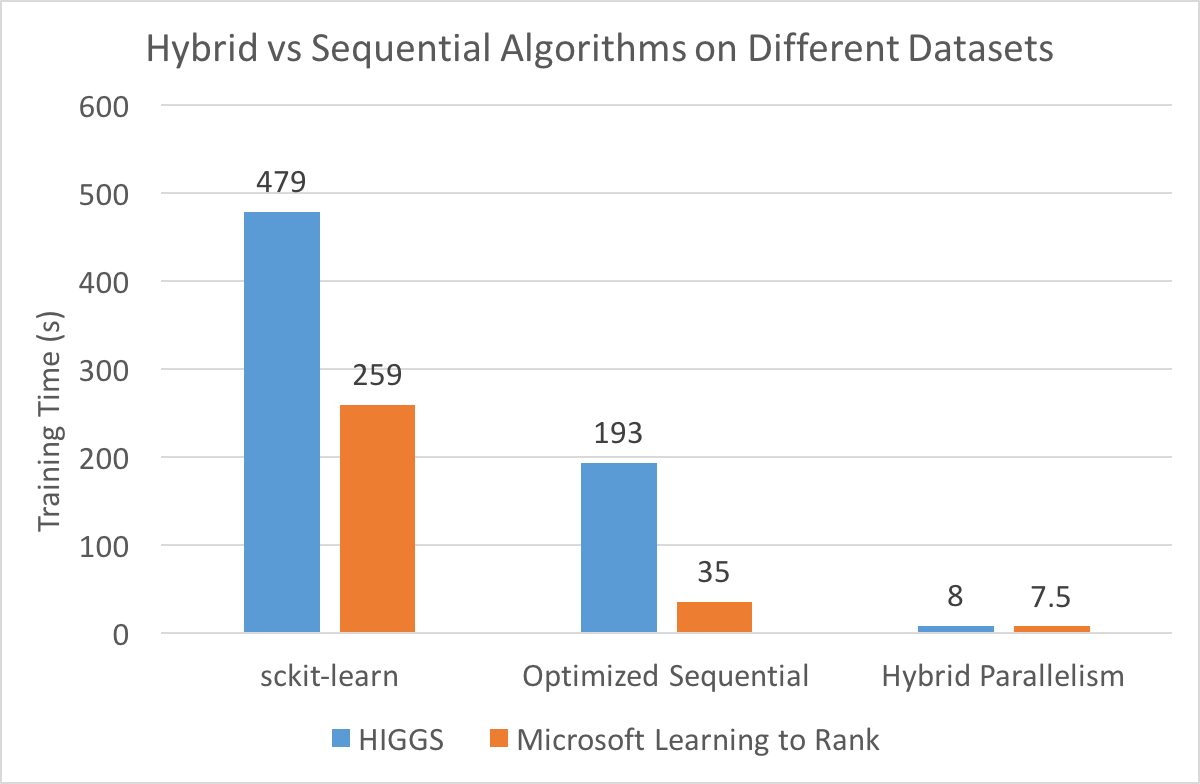
Based on our intial profiling, the hybrid algorithm benefits significantly from the increase in dataset size, supporting our hypothesis that a larger dataset would offset the CUDA memory setup overhead and allow a GPU/hybrid implementation to shine. Specifically, our hybrid implementation has a 24x speedup over our optimized sequential version for the HIGGs dataset, but only a 4.7x speedup when training on the Microsoft Learning to Rank dataset.
References
Picture sources:
https://upload.wikimedia.org/wikipedia/commons/f/f3/CART_tree_titanic_survivors.png
Papers:
Learning to Rank Using Classification and Gradient Boosting
https://www.microsoft.com/en-us/research/wp-content/uploads/2016/02/boosttreerank.pdf
A Communication-Efficient Parallel Algorithm for Decision Tree
https://arxiv.org/abs/1611.01276
Datasets:
HIGGS Classification Dataset
https://archive.ics.uci.edu/ml/datasets/HIGGS
Microsoft Learning to Rank Dataset
https://www.microsoft.com/en-us/research/project/mslr/
Libraries for Benchmarking:
Decision Trees Module in scikit-learn
http://scikit-learn.org/stable/modules/tree.html
Equal work was done by both project members.